Time-Continuous Neural Architectures

• irregularly measured time series
• previous solutions:
  • attach timestamps to observations
  • missing values -> GRU-D (informative missingness) link
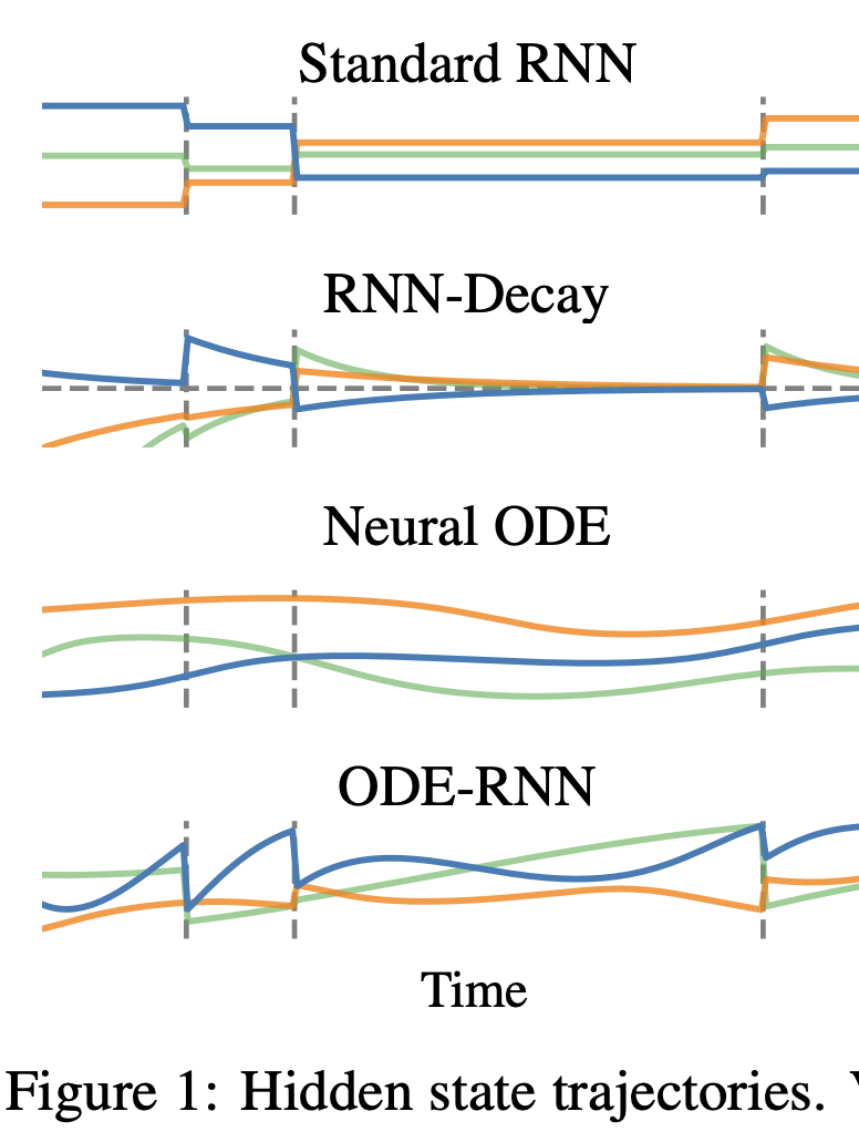
    • simple exponential decay between observations
• hidden state 𝑧(𝑡) ∈ 𝒵 that evolves continuously in time with potentially discontinuous updates when a new observation is made
• between two observation times, the hidden state evolves according to a set of flow curves
• explicitly modeling interventions? -> causality
• Training
  • Adjoint method
    • lower memory costs, less accurate
  • Backpropagation-Through-Time
    • vanishing/exploding gradients problem -> gates

Continuous-time recurrent neural networks

• any continuous curve can be approximated by the output of a recurrent neural network.
• outcome distribution 𝑃𝜽, neural networks: 𝑁𝑁𝑖𝑛𝑖𝑡, 𝑁𝑁𝑗𝑢𝑚𝑝, 𝑁𝑁𝑜𝑢𝑡 and flow 𝐹x,ϕ,
• initialization:
  • 𝑧(𝑡0 ) = 𝑁𝑁𝑖𝑛𝑖𝑡 (𝑥0 )
• Update: With new observation vector 𝒉𝑡 set:
  • 𝑧(𝑡) = 𝑁𝑁𝑗𝑢𝑚𝑝(𝒉𝒕 , 𝑧(𝑡−))
• Evolve:
  • 𝑧(𝑡 + Δ𝑡 ) = 𝐹x,ϕ(𝑧(𝑡),𝑡 + Δ𝑡 )
• Forecast
  • y = 𝜽 = 𝑁𝑁𝑜𝑢𝑡(𝑧(𝑡 + Δ𝑡))
• the distinctions lie in the architecture of the sub-networks and which inputs and hidden states are passed to the sub-networks!
• original article (hard-to-read) link

• article (overview) link

• CT-GRU:
  • replace the GRU storage (update gate) and retrieval (reset) gates with storage and retrieval scales, computed from the external input and the current hidden state
  • (context-dependent) time scale is expressed in terms of a time constant -> exponential decay
  • article (good intro) link
  • exponential decay dynamics did not improve predictive performance over standard RNN approaches
• CT-LSTM:
  • LSTM: input gate, forget gate, output gate
  • same approach
  • a decay term proportional to the time interval between events -> affects gates
  • article link

Neural ODEs

• instead of the hidden state parameterize the derivative of the hidden state
• treating the neural network as the solution to an ordinary differential equation
• model the vector field associated with the flow curves using a neural network
• 𝑑𝑧 / 𝑑𝑡 = 𝑁𝑁𝑣𝑒𝑐(𝑧(𝑡)),
• 𝑧(𝑡1 ) = 𝑧(0) + ∫ 𝑁𝑁𝑣𝑒𝑐(𝑧(𝑠))𝑑𝑠 -> ODE solver
• choice of ODE solver enables adaptive computation (speed <-> accuracy)

• article link

• article (10/10) link
• ODE-RNN:

  • neural ODE evolution of the hidden state between observations

    

• Autoregressive ODE models

  • p(x) = Product(i pθ(xi

    xi−1, . . . , x0))

  • simple ODE-RNN to predict next time step
  • dynamics and the conditioning on data are encoded implicitly through the hidden state updates
  • hard to interpret
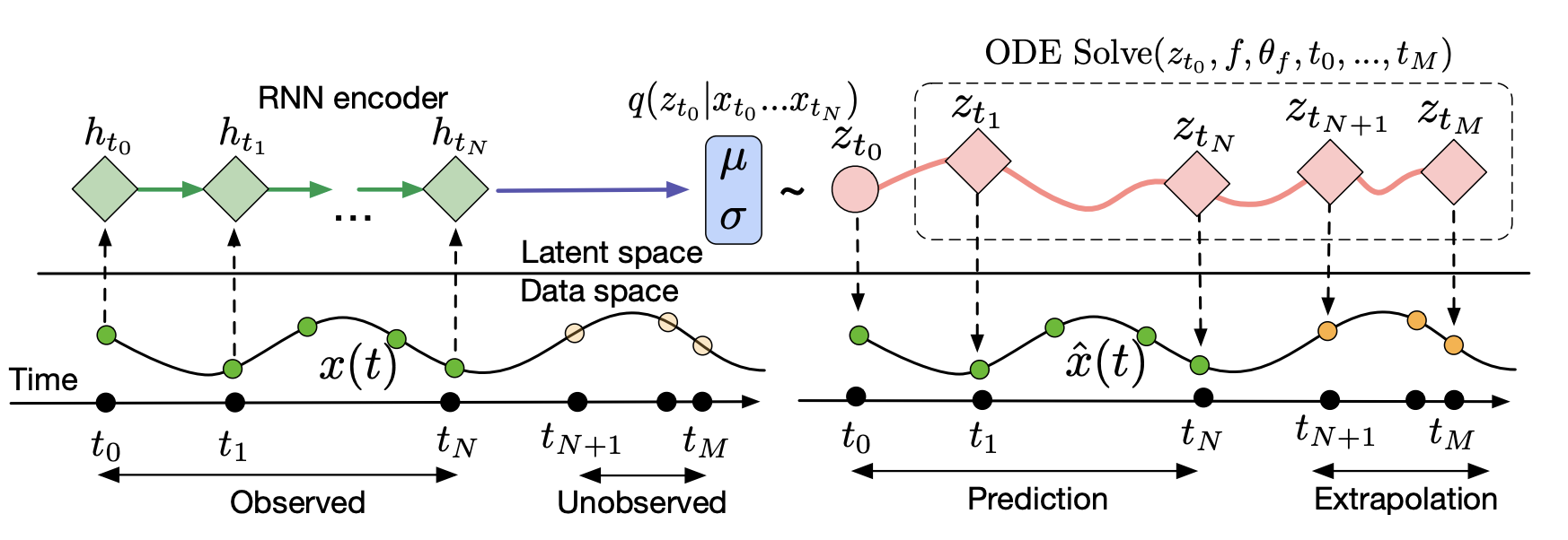
• Latent ODE
  • VAE-like structure/training
  • first: RNN recognition model
  • later: ODE-RNN recognition model -> better representation -> extrapolation
  • represents state explicitly through state
  • represent dynamics explicitly through a generative model
    • Latent states can be used to compare different time series, for e.g. clustering or classification tasks
    • dynamics functions can be examined to identify the types of dynamics present in the dataset

    

  • augmentation:
    • Poisson process to model observation frequency
• ODE-LSTM
  • LSTM ODE in recognition model
  • long-term dependencies
  • similar: GRU-ODE appeared in Latent ODE paper
    • evolve the hidden state h(t) with an ODE, until observe new xt1
    • use GRU-cell to update at that point
  • article (10/8) link
• improving performance:
  • semi-norm trick for faster backpropagation link
  • reparameterization trick for ODEs for faster mini-batching link

Neural flows

• different: Continuous Normalizing Flows (CNF)
  • normalizing flows video link
  • Neural ODEs: moving from a discrete set of layers to a continuous transformation simplifies the computation of the change in normalizing constant (Jacobian) -> efficiency
  • better accuracy, faster convergence, more interpretable normalizing flow models
  • stochastic estimation of trace (even more efficiency) link
  • attentive CNF: attention mechanism
• neural network to directly parameterize the flow curves
  • computational efficiency
• 𝑧(𝑡1 ) = 𝑁𝑁𝑓𝑙𝑜𝑤(𝑧(0), (𝑡0,𝑡1 ))
• condition: 𝑁𝑁𝑓𝑙𝑜𝑤 is invertible!
  • Linear Flow
    • F(t, x0) = exp(At)x0
  • ResNet Flow
    • F(t, x) = x + ϕ(t)(g(t, x))
    • ϕ(t): activation; g(t, x): neural network
    • residual layer xt+1 = xt + g(xt) -> resemblance to ODE-solve
  • GRU Flow
    • time series data
    • flow version of GRU-ODE: can be rewritten into the form of a single Residual layer
    • F(t, h) = h + r(t)(1 − z(t, h))  (c(t, h) − h)
    • append xt to the input of z, r and c -> a continuous-in-time version of GRU
  • Coupling Flow
    • ResNet flow, GRU flow -> missing analytical inverse
    • splitting the input dimensions into two disjoint sets A and B
    • F(t, x)A = xA exp(u(t, xB)ϕu(t)) + v(t, xB)ϕv(t)
  • ϕ or r : “time embedding function”
• Latent Variable models (VAE)
  • Encoder: ODE-LSTM with flow instead of ODESolve
  • Decoder: simply pass the next time point into F and get the next hidden state directly
• Continuous Normalizing Flows (CNF)
  • coupling flow allows for more efficient computation
• article link

Interesting Related Topics

• Augmented NODE, Second Order NODE link

• Temporal Point Processes: link
  • the times at which we observe the events come from some underlying process, which we model
  • Marked point processes: what type of an event happened
• Neural Jump Stochastic Differential Equations link

• Spatio-Temporal Point Processes: link

• Flow based models
  • normalizing flows
  • autoregressive flows link
  • matrix factorization based flow link
• Continually Learning Recurrent Neural Network link link

State-Space Models

video, idea

• Legendre Memory Units: Continuous-Time Representation in Recurrent Neural Networks link
• HiPPO: Recurrent Memory with Optimal Polynomial Projections link
• Statistical learning in human sensorimotor control video